2. Finding Spikes! — Analyzing Patch-Clamp Electrophysiology in Python

Note¶

This section primairly focuses using IPFX to analyze your patch clamp data. In particular focuses on analyzing current clamp data. However you may find success with other analysis packages such as https://github.com/BlueBrain/BluePyEfe

import numpy as np
import pandas as pd
import matplotlib.pyplot as plt
import pyabf
import ipfx
from IPython.display import display, HTML

C:\Users\SMest\Anaconda3\lib\site-packages\numpy\_distributor_init.py:32: UserWarning: loaded more than 1 DLL from .libs:
C:\Users\SMest\Anaconda3\lib\site-packages\numpy\.libs\libopenblas.NOIJJG62EMASZI6NYURL6JBKM4EVBGM7.gfortran-win_amd64.dll
C:\Users\SMest\Anaconda3\lib\site-packages\numpy\.libs\libopenblas.PYQHXLVVQ7VESDPUVUADXEVJOBGHJPAY.gfortran-win_amd64.dll
  stacklevel=1)
In C:\Users\SMest\Anaconda3\lib\site-packages\matplotlib\mpl-data\stylelib\_classic_test.mplstyle: 
The text.latex.preview rcparam was deprecated in Matplotlib 3.3 and will be removed two minor releases later.
In C:\Users\SMest\Anaconda3\lib\site-packages\matplotlib\mpl-data\stylelib\_classic_test.mplstyle: 
The mathtext.fallback_to_cm rcparam was deprecated in Matplotlib 3.3 and will be removed two minor releases later.
In C:\Users\SMest\Anaconda3\lib\site-packages\matplotlib\mpl-data\stylelib\_classic_test.mplstyle: Support for setting the 'mathtext.fallback_to_cm' rcParam is deprecated since 3.3 and will be removed two minor releases later; use 'mathtext.fallback : 'cm' instead.
In C:\Users\SMest\Anaconda3\lib\site-packages\matplotlib\mpl-data\stylelib\_classic_test.mplstyle: 
The validate_bool_maybe_none function was deprecated in Matplotlib 3.3 and will be removed two minor releases later.
In C:\Users\SMest\Anaconda3\lib\site-packages\matplotlib\mpl-data\stylelib\_classic_test.mplstyle: 
The savefig.jpeg_quality rcparam was deprecated in Matplotlib 3.3 and will be removed two minor releases later.
In C:\Users\SMest\Anaconda3\lib\site-packages\matplotlib\mpl-data\stylelib\_classic_test.mplstyle: 
The keymap.all_axes rcparam was deprecated in Matplotlib 3.3 and will be removed two minor releases later.
In C:\Users\SMest\Anaconda3\lib\site-packages\matplotlib\mpl-data\stylelib\_classic_test.mplstyle: 
The animation.avconv_path rcparam was deprecated in Matplotlib 3.3 and will be removed two minor releases later.
In C:\Users\SMest\Anaconda3\lib\site-packages\matplotlib\mpl-data\stylelib\_classic_test.mplstyle: 
The animation.avconv_args rcparam was deprecated in Matplotlib 3.3 and will be removed two minor releases later.

abf = pyabf.ABF("data/example1.abf") #this tells pyabf to load our data and store it in an abf object
abf.setSweep(7)

Setting up our spike finder¶

To begin with, we will import just the spike finder from IPFX.

from ipfx.feature_extractor import SpikeFeatureExtractor

Now we will create our SpikeFeatureExtractor. To do so, we will create a object similar to our ABF object. We can pass our settings to the object, that way we will not have to specify the settings repeatedly. More on this later

spike_fe = SpikeFeatureExtractor(filter=0) #Set the filter to 0

The above command intializes the spike feature extractor. Similar to the abf object, this has many attributes we can access.

dir(spike_fe)[-10:]

['max_interval',
 'min_height',
 'min_peak',
 'process',
 'reject_at_stim_start_interval',
 'spike_feature',
 'spike_feature_keys',
 'spikes',
 'start',
 'thresh_frac']

Getting the Spikes¶

To begin, we will use the spike.process function to find our data. This function takes our Time, Response, and Command waveforms as input.

spikes = spike_fe.process(abf.sweepX, abf.sweepY, abf.sweepC) #Processes that specific sweep from the ABF file

INFO:numexpr.utils:Note: NumExpr detected 16 cores but "NUMEXPR_MAX_THREADS" not set, so enforcing safe limit of 8.
INFO:numexpr.utils:NumExpr defaulting to 8 threads.

This returns a pandas dataframe containing information for each spike detected. These dataframes are similar to excel spread sheets. Each row is a single spike, and each column is a feature of that spike (for example peak voltage). For more explicit definitions of the various columns I recommend checking out the Allen Institutes Ephys Whitepaper. We can take a peek:

display(spikes)

	threshold_index	clipped	threshold_t	threshold_v	threshold_i	peak_index	peak_t	peak_v	peak_i	trough_index	...	adp_index	adp_t	adp_v	adp_i	slow_trough_index	slow_trough_t	slow_trough_v	slow_trough_i	width	upstroke_downstroke_ratio
0	12159	False	0.60795	-37.750244	50.0	12171	0.60855	27.832031	50.0	12214	...	NaN	NaN	NaN	NaN	12214.0	0.61070	-55.786133	50.0	0.00065	2.026667
1	12594	False	0.62970	-33.416748	50.0	12609	0.63045	18.920898	50.0	12671	...	NaN	NaN	NaN	NaN	12671.0	0.63355	-50.323486	50.0	0.00100	1.828125
2	12984	False	0.64920	-32.196045	50.0	13003	0.65015	14.862061	50.0	13072	...	NaN	NaN	NaN	NaN	13072.0	0.65360	-47.973633	50.0	0.00135	1.733333
3	13419	False	0.67095	-30.487061	50.0	13441	0.67205	14.953613	50.0	13524	...	NaN	NaN	NaN	NaN	13524.0	0.67620	-46.783447	50.0	0.00165	1.584416
4	13903	False	0.69515	-29.266357	50.0	13928	0.69640	13.366699	50.0	14021	...	NaN	NaN	NaN	NaN	14021.0	0.70105	-47.302246	50.0	0.00185	1.360000
5	14425	False	0.72125	-29.541016	50.0	14452	0.72260	15.319824	50.0	14544	...	NaN	NaN	NaN	NaN	14544.0	0.72720	-47.851562	50.0	0.00185	1.378378
6	15025	False	0.75125	-28.442383	50.0	15053	0.75265	13.885498	50.0	15154	...	NaN	NaN	NaN	NaN	15154.0	0.75770	-48.431396	50.0	0.00205	1.250000
7	15629	False	0.78145	-28.167725	50.0	15653	0.78265	15.869141	50.0	15762	...	NaN	NaN	NaN	NaN	15762.0	0.78810	-47.882080	50.0	0.00185	1.351351
8	16253	False	0.81265	-29.479980	50.0	16279	0.81395	16.082764	50.0	16376	...	NaN	NaN	NaN	NaN	16376.0	0.81880	-47.546387	50.0	0.00190	1.544118
9	16889	False	0.84445	-29.174805	50.0	16916	0.84580	14.495850	50.0	17036	...	NaN	NaN	NaN	NaN	17036.0	0.85180	-47.882080	50.0	0.00205	1.362319
10	17596	False	0.87980	-29.388428	50.0	17624	0.88120	14.190674	50.0	17752	...	NaN	NaN	NaN	NaN	17752.0	0.88760	-46.539307	50.0	0.00205	1.375000
11	18320	False	0.91600	-29.510498	50.0	18348	0.91740	16.571045	50.0	18447	...	NaN	NaN	NaN	NaN	18447.0	0.92235	-47.882080	50.0	0.00195	1.304348
12	19073	False	0.95365	-28.686523	50.0	19099	0.95495	15.869141	50.0	19226	...	NaN	NaN	NaN	NaN	19226.0	0.96130	-47.210693	50.0	0.00200	1.319445
13	19825	False	0.99125	-28.442383	50.0	19855	0.99275	16.021729	50.0	19984	...	NaN	NaN	NaN	NaN	19984.0	0.99920	-48.217773	50.0	0.00210	1.197183
14	20628	False	1.03140	-28.015137	50.0	20657	1.03285	15.686035	50.0	20802	...	NaN	NaN	NaN	NaN	20802.0	1.04010	-47.485352	50.0	0.00210	1.269841
15	21393	False	1.06965	-29.083252	50.0	21421	1.07105	16.784668	50.0	21559	...	NaN	NaN	NaN	NaN	21559.0	1.07795	-48.370361	50.0	0.00210	1.358209
16	22095	False	1.10475	-28.625488	50.0	22120	1.10600	16.906738	50.0	22250	...	NaN	NaN	NaN	NaN	22250.0	1.11250	-46.417236	50.0	0.00200	1.575758
17	22840	False	1.14200	-30.029297	50.0	22870	1.14350	17.242432	50.0	22998	...	NaN	NaN	NaN	NaN	22998.0	1.14990	-49.102783	50.0	0.00210	1.277778
18	23567	False	1.17835	-29.602051	50.0	23596	1.17980	15.441895	50.0	23729	...	NaN	NaN	NaN	NaN	23729.0	1.18645	-47.515869	50.0	0.00215	1.507692
19	24286	False	1.21430	-29.968262	50.0	24317	1.21585	15.594482	50.0	24460	...	NaN	NaN	NaN	NaN	24460.0	1.22300	-47.668457	50.0	0.00210	1.444444
20	24936	False	1.24680	-29.876709	50.0	24966	1.24830	15.747070	50.0	44707	...	NaN	NaN	NaN	NaN	NaN	NaN	NaN	NaN	0.00215	1.550000

21 rows × 36 columns

We can also visualize the detected spikes on a plot:

#isolate the columns for plotting
spike_times = spikes['peak_t'] #This isolates the peak_t columm
spike_peak = spikes['peak_v'] #this isolates the peak_v column
sweepX = abf.sweepX
sweepY = abf.sweepY
sweepC = abf.sweepC
#Create a figure
plt.figure(1)
plt.plot(sweepX, sweepY)
plt.scatter(spike_times, spike_peak, c='r', marker='x') #Plots X's at the peak of the action potential
plt.xlabel("Time (s)")
plt.ylabel(abf.sweepLabelY) #
plt.xlim(0.55, 1.5)

(0.55, 1.5)

The pandas dataframe contains a number of useful functions for analysis. For example we can take the mean of a column

mean_trough = spikes['fast_trough_v'].mean()
print(f"Found a mean trough of {mean_trough}")

Found a mean trough of -44.91751480102539

In addition we can save the dataframe for opening later:

spikes.to_csv("out.csv") #Outputs the dataframe to a csv for opening in excel
#The "out.csv" specifies the file location/name

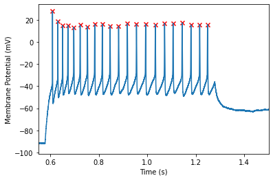
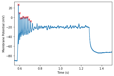
Ensuring you captures the spikes¶

The above example uses the default spike finding options. This is suitable for many applications. However, one may find that this over/under detects spikes in your data. Take for example, the spikes found in one of the latter sweeps:

abf.setSweep(14)
spikes = spike_fe.process(abf.sweepX, abf.sweepY, abf.sweepC)

#isolate the columns for plotting
spike_times = spikes['peak_t'] #This isolates the peak_t columm
spike_peak = spikes['peak_v'] #this isolates the peak_v column
sweepX = abf.sweepX
sweepY = abf.sweepY
sweepC = abf.sweepC
#Create a figure
plt.figure(1)
plt.plot(sweepX, sweepY)
plt.scatter(spike_times, spike_peak, c='r', marker='x') #Plots X's at the peak of the action potential
plt.xlabel("Time (s)")
plt.ylabel(abf.sweepLabelY) #
plt.xlim(0.55, 1.5)

(0.55, 1.5)

It still catches most of the spikes, however, it misses one or two spikes at the end of the train that you may want to pick up. To ensure we pick up these spikes, we can adjust a few parameters available to us. We can view the available options here:

help(spike_fe)

Help on SpikeFeatureExtractor in module ipfx.feature_extractor object:

class SpikeFeatureExtractor(builtins.object)
 |  SpikeFeatureExtractor(start=None, end=None, filter=10.0, dv_cutoff=20.0, max_interval=0.005, min_height=2.0, min_peak=-30.0, thresh_frac=0.05, reject_at_stim_start_interval=0)
 |  
 |  Methods defined here:
 |  
 |  __init__(self, start=None, end=None, filter=10.0, dv_cutoff=20.0, max_interval=0.005, min_height=2.0, min_peak=-30.0, thresh_frac=0.05, reject_at_stim_start_interval=0)
 |      Initialize SweepFeatures object.-
 |      
 |      Parameters
 |      ----------
 |      t : ndarray of times (seconds)
 |      v : ndarray of voltages (mV)
 |      i : ndarray of currents (pA)
 |      start : start of time window for feature analysis (optional)
 |      end : end of time window for feature analysis (optional)
 |      filter : cutoff frequency for 4-pole low-pass Bessel filter in kHz (optional, default 10)
 |      dv_cutoff : minimum dV/dt to qualify as a spike in V/s (optional, default 20)
 |      max_interval : maximum acceptable time between start of spike and time of peak in sec (optional, default 0.005)
 |      min_height : minimum acceptable height from threshold to peak in mV (optional, default 2)
 |      min_peak : minimum acceptable absolute peak level in mV (optional, default -30)
 |      thresh_frac : fraction of average upstroke for threshold calculation (optional, default 0.05)
 |      reject_at_stim_start_interval : duration of window after start to reject potential spikes (optional, default 0)
 |  
 |  is_spike_feature_affected_by_clipping(self, key)
 |  
 |  process(self, t, v, i)
 |  
 |  spike_feature(self, spikes_df, key, include_clipped=False, force_exclude_clipped=False)
 |      Get specified feature for every spike.
 |      
 |      Parameters
 |      ----------
 |      key : feature name
 |      include_clipped: return values for every identified spike, even when clipping means they will be incorrect/undefined
 |      
 |      Returns
 |      -------
 |      spike_feature_values : ndarray of features for each spike
 |  
 |  spike_feature_keys(self, spikes_df)
 |      Get list of every available spike feature.
 |  
 |  spikes(self, spikes_df)
 |      Get all features for each spike as a list of records.
 |  
 |  ----------------------------------------------------------------------
 |  Data descriptors defined here:
 |  
 |  __dict__
 |      dictionary for instance variables (if defined)
 |  
 |  __weakref__
 |      list of weak references to the object (if defined)
 |  
 |  ----------------------------------------------------------------------
 |  Data and other attributes defined here:
 |  
 |  AFFECTED_BY_CLIPPING = ['trough_t', 'trough_v', 'trough_i', 'trough_in...

First, we will take a look at the dv/dt threshold!

dv_cutoff: dV/dT threshold¶

The dV/dT threshold is the primary method by which ipfx detects spikes. Putative spikes must pass this check prior to any other settings being applied. By default, ipfx looks for points at which the dV/dT crosses 20mV/mS (V/s) (based on the ephys whitepaper noted above). if we examine the dV/dt of our trace, we can see that the smaller spikes do not reach this threshold

dV = np.diff(abf.sweepY) #take the difference of the adjacent points in mV
dT = np.diff(abf.sweepX * 1000) #take the difference of adjacent points in s * 1000 -> ms
dvdt = dV/dT #compute dvdt in mV/ms -> v/s
plt.plot(abf.sweepX[:-1], dvdt)
plt.xlim(0.55, 0.8)
plt.axhline(20, label='20mV/ms', c='r') #plot a horizontal line at 20mV/ms
plt.axhline(10, label='10mV/ms', c='g') #plot a horizontal line at 20mV/ms
plt.legend()

<matplotlib.legend.Legend at 0x2a9e66cfa58>

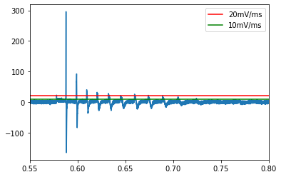
However, it appears that setting a threshold of 10mV/ms should do the trick! Now we will reinitialize the spike finder with the new threshold

spike_fe = SpikeFeatureExtractor(filter=0, dv_cutoff=10) #reintialize with a dv threshold of 10
spikes = spike_fe.process(abf.sweepX, abf.sweepY, abf.sweepC)

#isolate the columns for plotting
spike_times = spikes['peak_t'] #This isolates the peak_t columm
spike_peak = spikes['peak_v'] #this isolates the peak_v column
sweepX = abf.sweepX
sweepY = abf.sweepY
sweepC = abf.sweepC
#Create a figure
plt.figure(1)
plt.plot(sweepX, sweepY)
plt.scatter(spike_times, spike_peak, c='r', marker='x') #Plots X's at the peak of the action potential
plt.xlabel("Time (s)")
plt.ylabel(abf.sweepLabelY) #
plt.xlim(0.55, 1.5)

(0.55, 1.5)

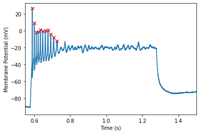
Its looking good! However, lets say we decided to exclude the final spike in the train, we can adjust some of the other parameters to do so.

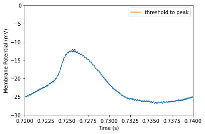
max_interval: Time between threshold and peak¶

Max interval defines the maximum length of time between the detected threshold and the detected peak. In many cases the default (5ms) should be fine. However, if you have slow or oddly shaped spikes, you may find adjusting this parameter useful. Take for example our threshold to peak time from our last sweep.

#isolate the columns for plotting
spike_times = spikes['peak_t'] #This isolates the peak_t columm
spike_peak = spikes['peak_v'] #this isolates the peak_v column
final_spike = spikes['peak_t'].to_numpy()[-1] #Gets the time of the last peak
final_threshold = spikes['threshold_t'].to_numpy()[-1] #gets the last threshgold
time = final_spike - final_threshold
print(f"Threshold to peak time of {time*1000}ms")

Threshold to peak time of 1.6499999999999293ms

sweepX = abf.sweepX
sweepY = abf.sweepY
sweepC = abf.sweepC
#Create a figure
plt.figure(1)
plt.plot(sweepX, sweepY)
plt.scatter(spike_times, spike_peak, c='r', marker='x') #Plots X's at the peak of the action potential
plt.plot(np.linspace(final_threshold, final_spike, 10), np.full(10, -20), label="threshold to peak")
plt.xlabel("Time (s)")
plt.legend()
plt.ylabel(abf.sweepLabelY) #
plt.xlim(0.72, 0.74)
plt.ylim(-30, 0)

(-30.0, 0.0)

By specifying the threshold-to-peak time we can drop this spike

spike_fe = SpikeFeatureExtractor(filter=0, dv_cutoff=10, max_interval=0.00164) #Note that the units are in seconds
spikes = spike_fe.process(abf.sweepX, abf.sweepY, abf.sweepC)

INFO:root:Need to recalculate threshold-peak pair that exceeds maximum allowed interval (0.001640 s)
INFO:root:Need to recalculate threshold-peak pair that exceeds maximum allowed interval (0.001640 s)
INFO:root:Need to recalculate threshold-peak pair that exceeds maximum allowed interval (0.001640 s)
INFO:root:Need to recalculate threshold-peak pair that exceeds maximum allowed interval (0.001640 s)
INFO:root:Need to recalculate threshold-peak pair that exceeds maximum allowed interval (0.001640 s)
INFO:root:Need to recalculate threshold-peak pair that exceeds maximum allowed interval (0.001640 s)
INFO:root:Need to recalculate threshold-peak pair that exceeds maximum allowed interval (0.001640 s)
INFO:root:Could not redetermine threshold-peak pair - dropping that pair
INFO:root:Could not redetermine threshold-peak pair - dropping that pair
INFO:root:Could not redetermine threshold-peak pair - dropping that pair
INFO:root:Could not redetermine threshold-peak pair - dropping that pair
INFO:root:Could not redetermine threshold-peak pair - dropping that pair
INFO:root:Could not redetermine threshold-peak pair - dropping that pair
INFO:root:Could not redetermine threshold-peak pair - dropping that pair

#isolate the columns for plotting
spike_times = spikes['peak_t'] #This isolates the peak_t columm
spike_peak = spikes['peak_v'] #this isolates the peak_v column
sweepX = abf.sweepX
sweepY = abf.sweepY
sweepC = abf.sweepC
#Create a figure
plt.figure(1)
plt.plot(sweepX, sweepY)
plt.scatter(spike_times, spike_peak, c='r', marker='x') #Plots X's at the peak of the action potential
plt.xlabel("Time (s)")
plt.ylabel(abf.sweepLabelY) #
plt.xlim(0.55, 1.5)

(0.55, 1.5)

Note that while we dropped that final spike, we lost other spikes! To remedy this, we can try adjusting the minimum height instead!

min_height: the minimum height between threshold and peak¶

The min height parameter defines the cutoff for the minimum amount of voltage an action potential must swing upward. This is computed as the difference between the peak and threshold. Therefore we will want to enter an absolute (non-negative) value. AP’s with a height below this value will be rejected. This value defaults of 2mV.

spike_fe = SpikeFeatureExtractor(filter=0, dv_cutoff=10, min_height=5) #reintialize with a min height of 5
spikes = spike_fe.process(abf.sweepX, abf.sweepY, abf.sweepC)

#isolate the columns for plotting
spike_times = spikes['peak_t'] #This isolates the peak_t columm
spike_peak = spikes['peak_v'] #this isolates the peak_v column
sweepX = abf.sweepX
sweepY = abf.sweepY
sweepC = abf.sweepC
#Create a figure
plt.figure(1)
plt.plot(sweepX, sweepY)
plt.scatter(spike_times, spike_peak, c='r', marker='x') #Plots X's at the peak of the action potential
plt.xlabel("Time (s)")
plt.ylabel(abf.sweepLabelY) #
plt.xlim(0.55, 1.5)

(0.55, 1.5)

We can see that we have successfully excluded the last spike. If we examine closer we can examine the heights of the action potentials

spike_fe = SpikeFeatureExtractor(filter=0, dv_cutoff=10) #reintialize with a min height of 5
spikes = spike_fe.process(abf.sweepX, abf.sweepY, abf.sweepC)

#isolate the columns for plotting
spike_times = spikes['peak_t'] #This isolates the peak_t columm
spike_peak = spikes['peak_v'] #this isolates the peak_v column
final_spike = spikes['peak_v'].to_numpy()[-1] #Gets the time of the last peak
final_threshold = spikes['threshold_v'].to_numpy()[-1] #gets the last threshgold
height = final_spike - final_threshold

sweepX = abf.sweepX
sweepY = abf.sweepY
sweepC = abf.sweepC
#Create a figure
plt.figure(1)
plt.plot(sweepX, sweepY)
plt.scatter(spike_times, spike_peak, c='r', marker='x') #Plots X's at the peak of the action potential
plt.plot(np.full(10, spike_times.to_numpy()[-1]),np.linspace(final_threshold, final_spike, 10), label="threshold to peak")
plt.xlabel("Time (s)")
plt.legend
plt.ylabel(abf.sweepLabelY) #
plt.xlim(0.72, 0.74)
plt.ylim(-30, 0)

(-30.0, 0.0)

min_peak: the minimum absolute peak of the action potential¶

Similar to the setting above, we can set the cutoff for the min peak of the action potential. However, this value is not calculated in reference to the threshold, instead, it is computed as the minimum the peak must reach (regardless of distance between peak and threshold). Therefore, its okay to use negative numbers for this setting. Action potentials with peaks that do not reach this level will be rejected. This value defaults to -30

spike_fe = SpikeFeatureExtractor(filter=0, dv_cutoff=10, min_peak=-10) #reintialize with a min peak 10
spikes = spike_fe.process(abf.sweepX, abf.sweepY, abf.sweepC)

#isolate the columns for plotting
spike_times = spikes['peak_t'] #This isolates the peak_t columm
spike_peak = spikes['peak_v'] #this isolates the peak_v column
sweepX = abf.sweepX
sweepY = abf.sweepY
sweepC = abf.sweepC
#Create a figure
plt.figure(1)
plt.plot(sweepX, sweepY)
plt.scatter(spike_times, spike_peak, c='r', marker='x') #Plots X's at the peak of the action potential
plt.xlabel("Time (s)")
plt.axhline(-10, label="min_peak threshold of -10")
plt.ylabel(abf.sweepLabelY) 
plt.xlim(0.55, 1.5)

(0.55, 1.5)

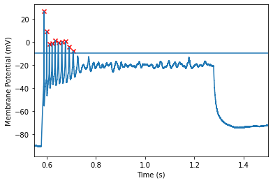
zooming a bit closer shows us that this threshold of -10 allows us to exclude the last spike but keep the others!

Putting it all together: Find spikes across all sweeps¶

So far we have just been analyzing a single sweep of our ABF file. However functionally

Analyzing Patch-Clamp Electrophysiology in Python

2. Finding Spikes!¶